2 Manuals
2.1 Build your own chart
This app allows you to plot a number of different node variables for the entire LN either as a histogram or as a scatter plot.
2.1.1 Histograms
The histogram app will let you plot a single variable from the “Choose a node variable” drop-down menu. Minimum and maximum values can be set to refine your searches since outliers can skew the distribution. For example, let’s look at the distribution of each node’s mean outbound fee rate (in ppm) across the LN.
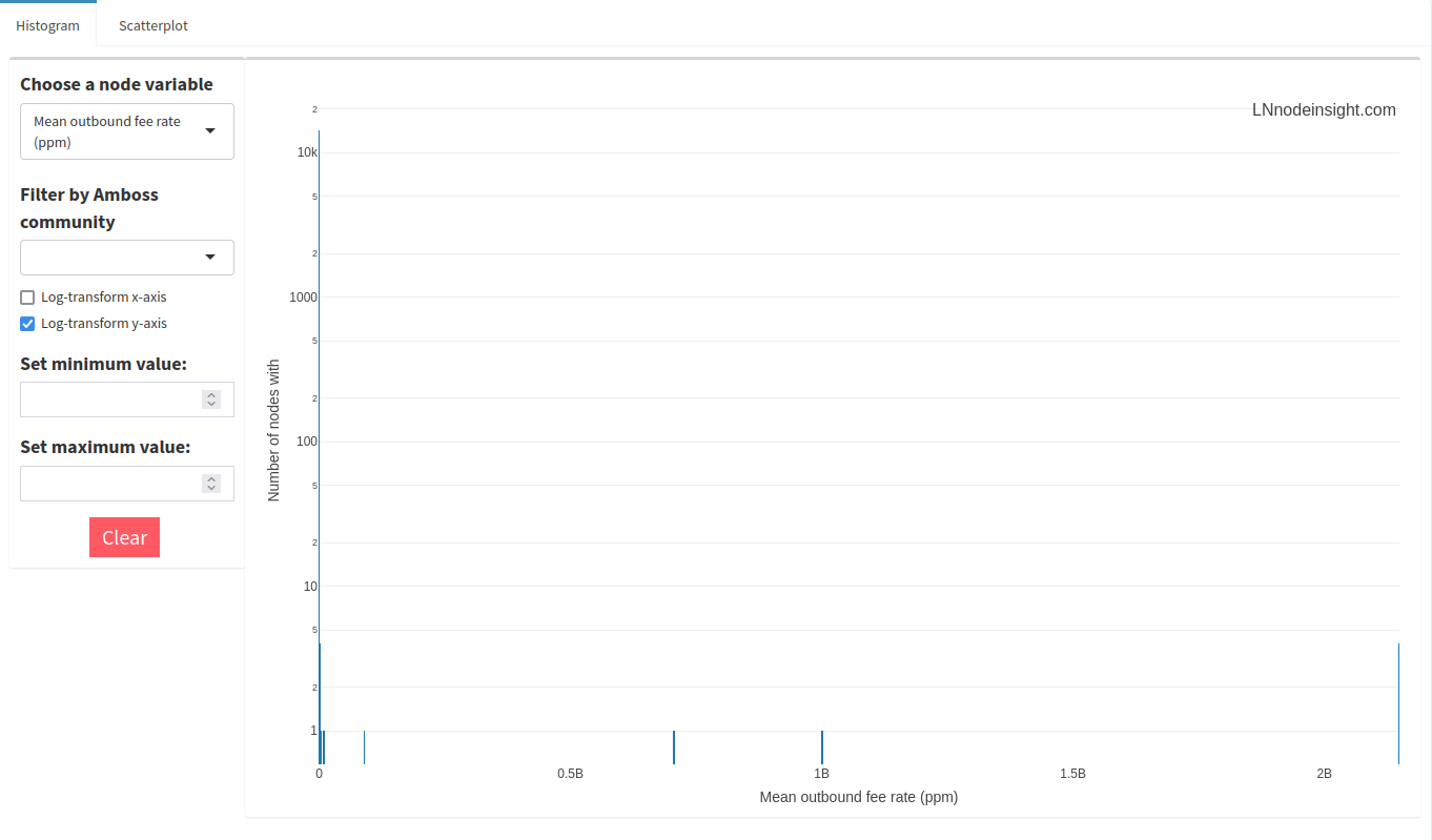
Not terribly insightful, is it? That’s because many nodes will implement extremely high fees to a peer where liquidity is exhausted to prevent forwarding failures. It’s fairly uncommon to see economically active fees toward any given node beyond 10 000ppm. Let’s apply that filter.
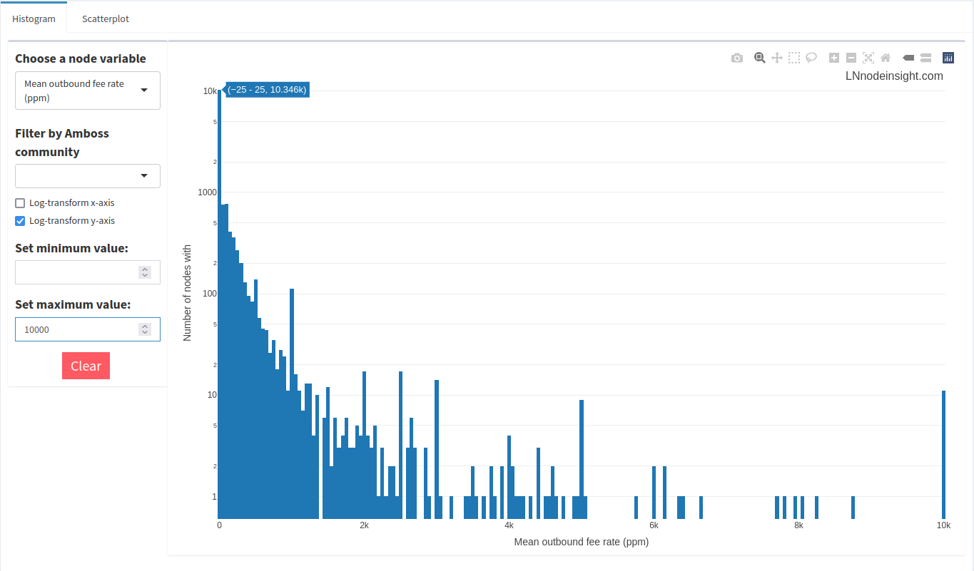
Much better! You can mouse over the bars to see which fee rates fall into that given bin. In the image, the mouse is over the very first bin, which indicates that around 10 300 nodes have average outbound fee rates between 0 and 25ppm. So, roughly 2/3 of all nodes on the network charge effectively nothing to forward a payment. That sounds great in theory, but in practice channels with such low fees usually have their liquidity drained, or the node operator is deliberately trying to encourage forwards to that peer, most likely because it is a liquidity source.
We can go layer on a social component by filtering the data according to an Amboss community. Let’s have a look at the Nodestrich community of node operators actively on Nostr.
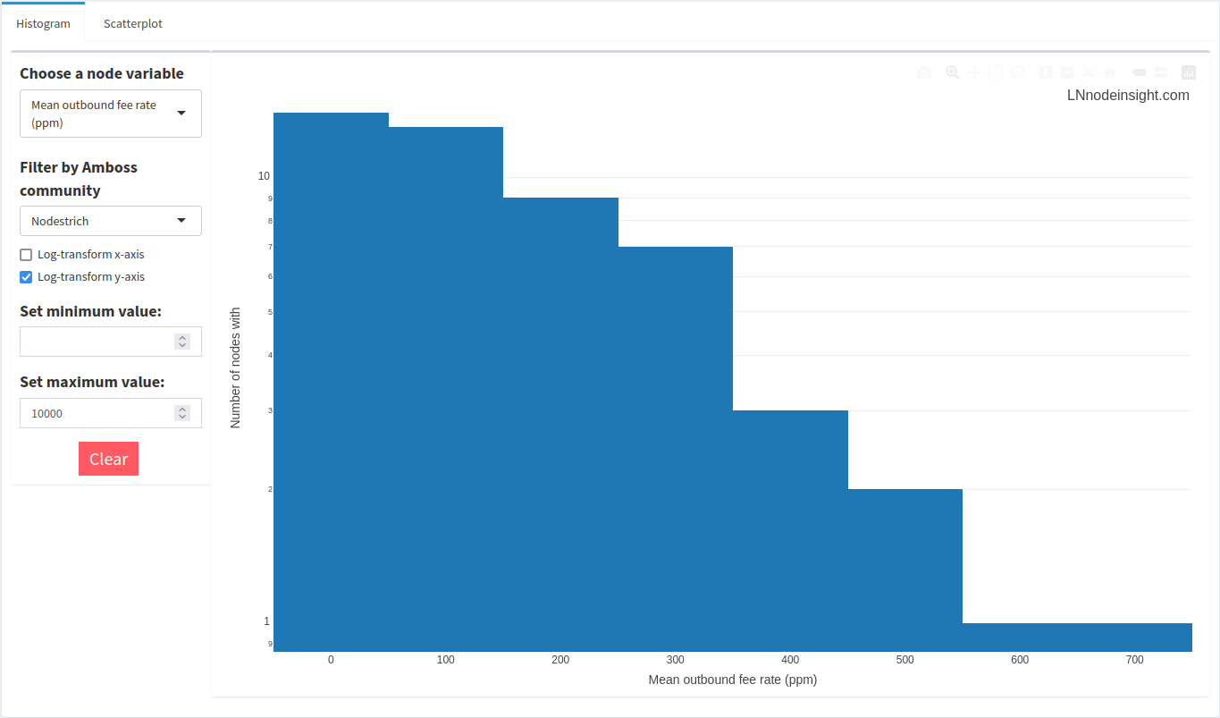
Most nodes in the community charge a nominal outbound fee, on average. Zap away at virtually no cost!
2.1.2 Scatter plots
The scatter plot app will let you plot two node variables together, which is often useful to spot relationships. You’ll need to select both an “X-axis variable” and a “Y-axis variable” from their respective drop-down menus to start off. For example, let’s plot a node’s average outbound fee to its corresponding total capacity.
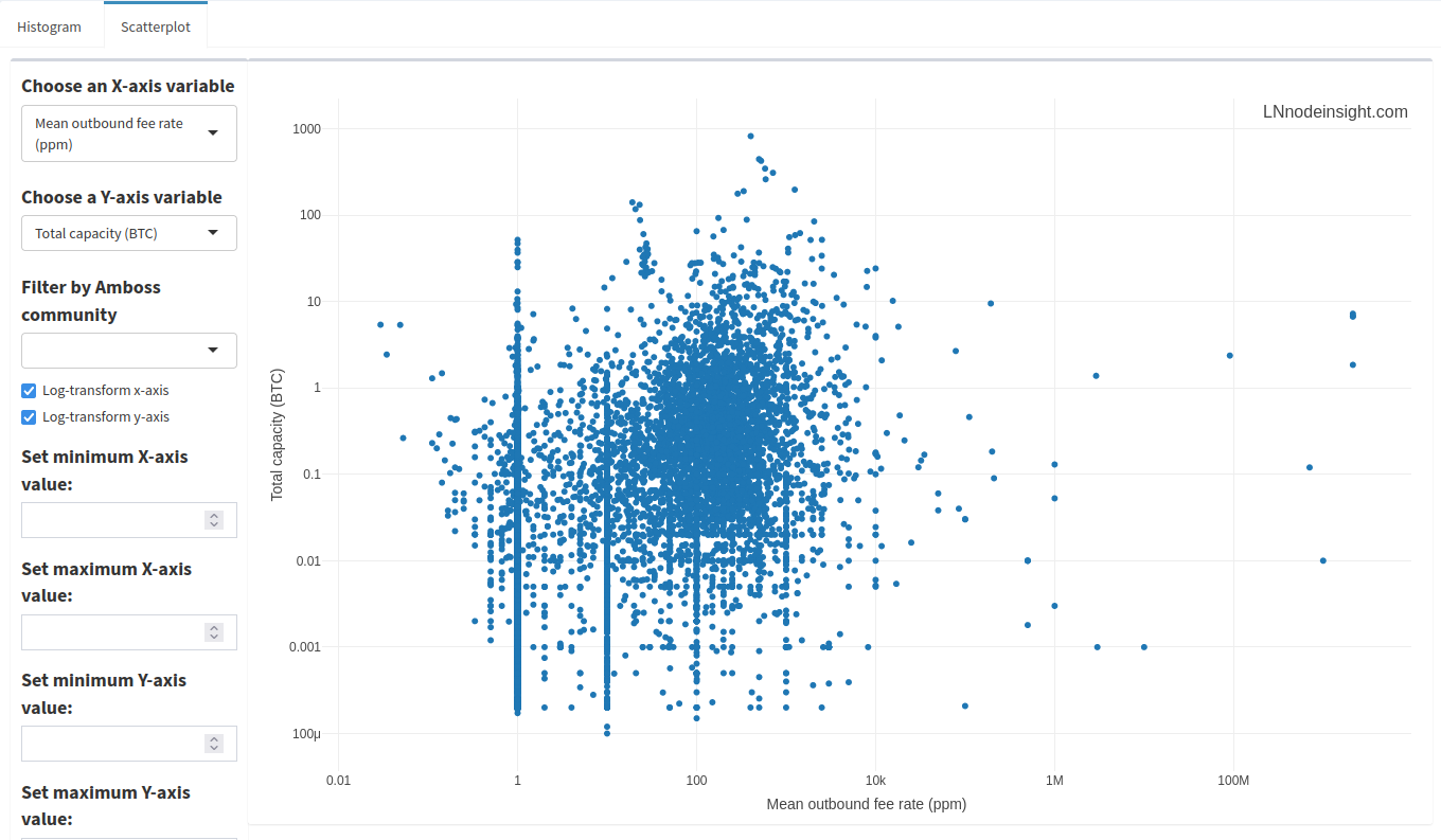
Just like with the histograms, there are a number of outlier data points where fees exceed 10 000ppm. We can filter just the same by removing those nodes whose average outbound fee rate is above 10 000ppm.
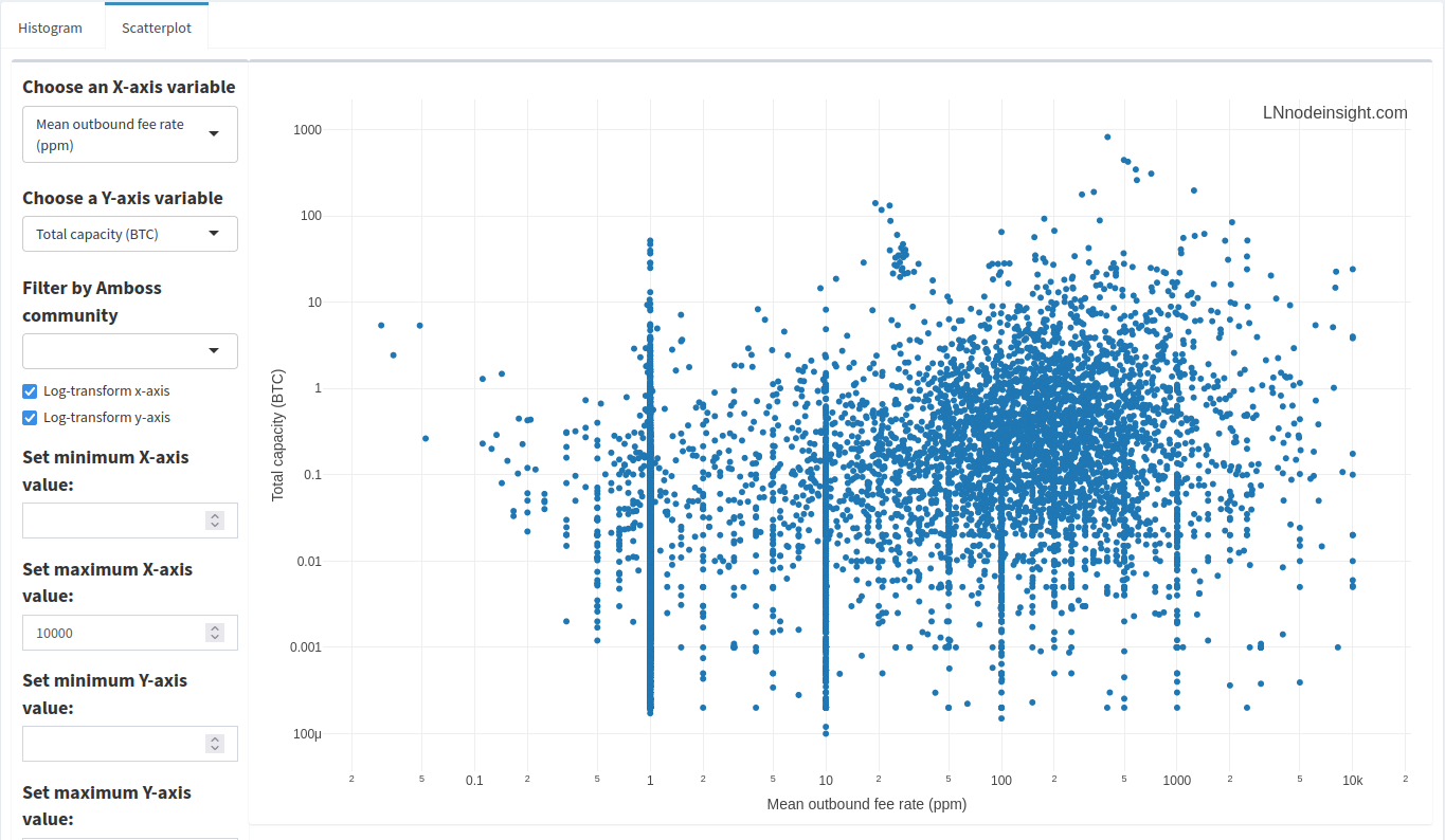
A little cleaner! Spot the trend here? Look at the stacks of points at very specific fee rates over a range of total capacities. The most prominent stacks are at 1, 10, 100 and 1000 ppm, with lesser ones at 5, 50 and 500 ppm. 1ppm is the default setting, so it looks like many nodes don’t bother to change that. However, the other points are just evidence that people like clean, round numbers. There’s lots of data in between those round numbers, so how would a node operator settle on such a value? Node operators are keen to automate a lot of the manual tasks around maintaining the node, and will set up rules to automate fee settings. Those rules might be based on channel balance, or the liquidity flow rate.
2.2 Node stats
2.2.1 Ranks
Drilling down into can reveal a lot about a node. A number of other venues offer this kind of node exploration, notably Amboss. Rather than repeat the same types of information, LNnodeInsight provides a number of unique and complementary views.
The first two sections display current centrality ranks, as well as historical ranks for the past 3 months plotted onto the same graph (visible for a small fee or unlimited with a subscription). Here’s an example:
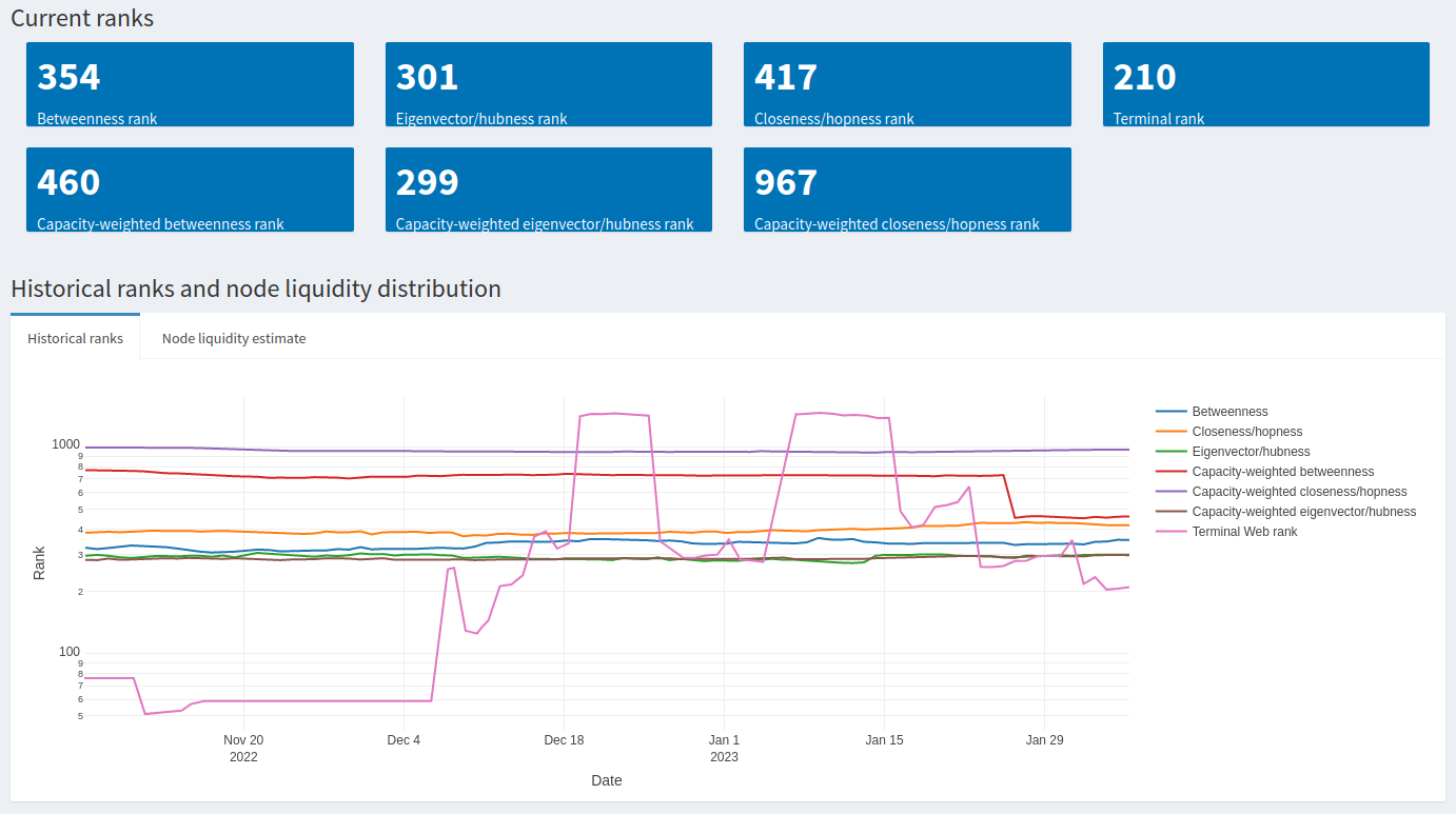
In thise case, some of this node’s ranks appear to change drastically while others don’t. Let’s take a closer look by highlighting only Betweenness, Closeness, Eigenvector centralities with the Lightning Terminal ranks.
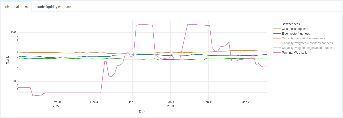
We can see that the centrality ranks really haven’t changed much over a 3 month period, whereas the Lightning Terminal rank appears volatile, particularly after December 6th, 2022. What does this mean? During the whole time period, this node’s channel peers haven’t changed much, and given the stability and range of centrality ranks this is a reasonably well situated node in the LN. There was also speculation around early December that Lightning Labs had modified its (hidden and closed-source) algorithm to rank nodes. Despite that, the node in question appears to be relatively stable. We can also examine the Node Liquidity Estimate tab (bundled together with historical ranks) to get an idea of how well this node maintains adequate liquidity where it is needed on its channels.
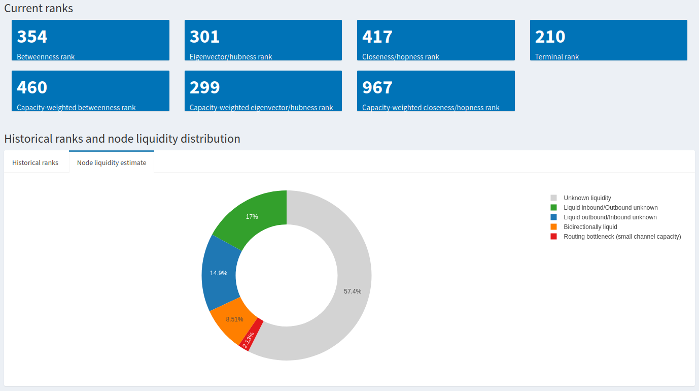
By nature it’s difficult to get a full picture of a node’s liquidity balance (in both channel directions) without them revealing all of that information, but we can nonetheless make some reasonable assumptions about the limited information available. The data collected to build this donut chart comes from liquidity tests over a period of two weeks. In this case, around 8.5% of the node’s channels are known to be liquid in both directions, whereas 17% are known to have inbound liquidity and around 15% have adequate outbound liquidity. Only a tiny fraction are small channels that often end up as routing bottlenecks. In sum, roughly 40% of this node’s channels were known to successfully respond to a liquidity request. This would suggest a relatively well-managed node.
2.2.2 Node averages compared to the whole LN
This section of the Node Stats page provides insight into how the node compares to the rest of the LN. For example, we can see how a node’s total capacity has changed over the past 3 months with respect to the LN.
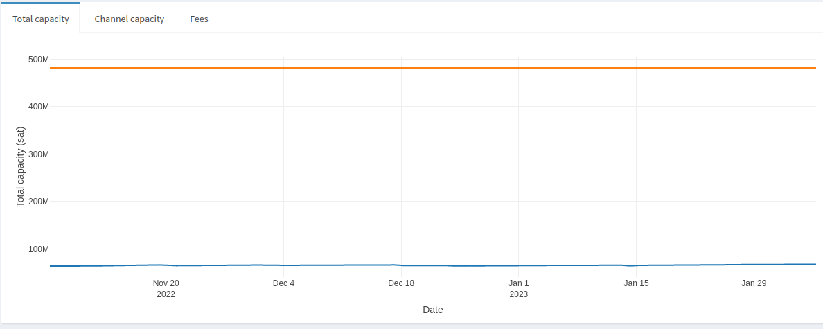
We can see that this node’s total capacity has remained under 500M sats over the whole period, and the average node’s capacity over the LN has also remained relatively static, at around 60M sats. This might be useful to know if looking for relatively stable peers. On the other hand, if you’re interested in identifying nodes actively growing then you would want to look for drastic increases in total capacity in a given time frame. Or you might want to avoid nodes that have been steadily decreasing their total capacity.
Aside from total capacity, we can look at a node’s average channel capacity compared to the LN channel average.
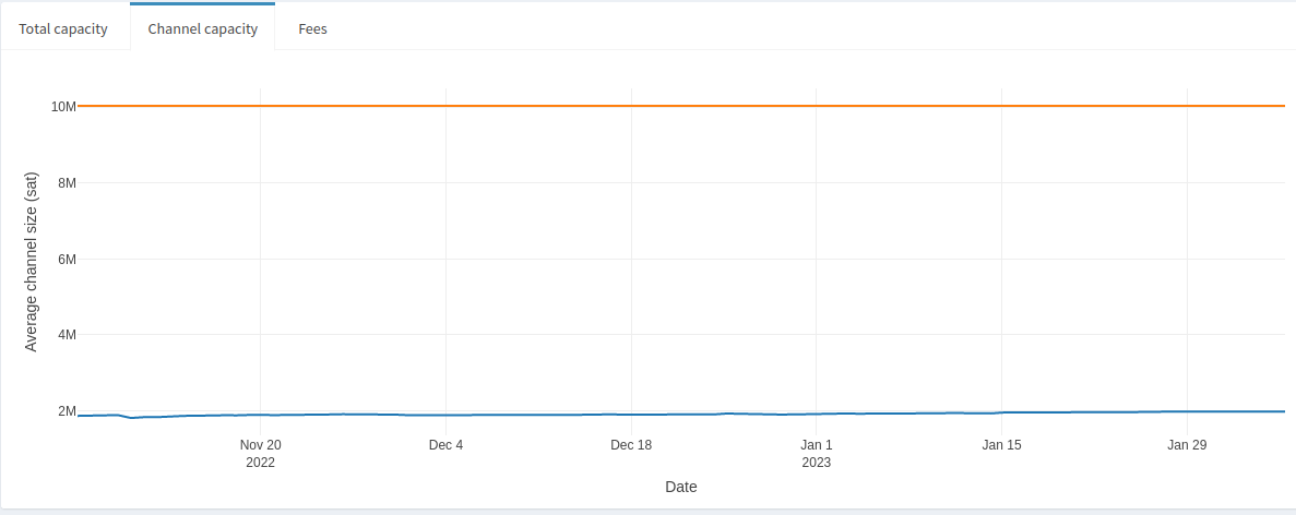
Not surprisingly this node’s average channel capacity has not changed since we know its total capacity has not changed. It’s currently sitting at 10M, more than 5x the average LN channel size. Relatively large channel sizes, in combination with well-managed liquidity, is usually a good sign that a node would make for a good peer–but these aren’t the only criteria! We can also look at the node’s average inbound and outbound fees compared to the LN average.
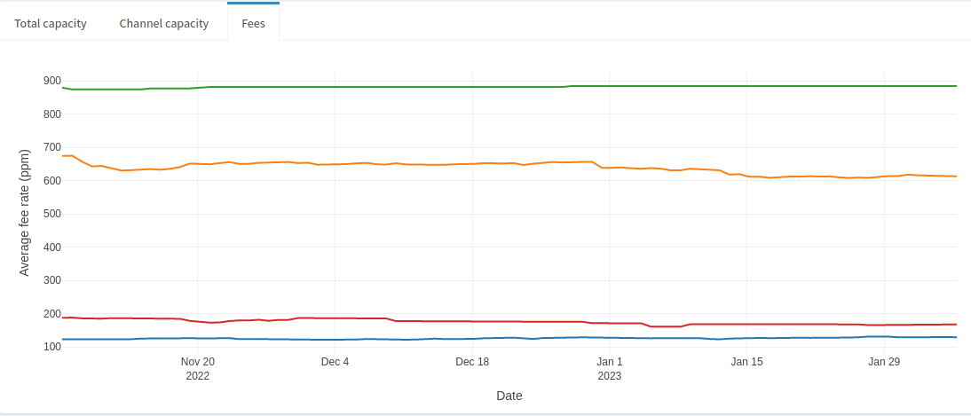
Here we can see that the node’s average outbound fees (in green) are just under 900ppm whereas its average inbound fee rate is around 200ppm. The average LN outbound fee rate is around 130ppm, but it’s average inbound is around 650ppm (skewed by some extreme outliers). This node charges more than 4x the cost to send a payment compared to its peers sending to it, and almost 7x compared to the average. It’s a more expensive node, which usually signals that active rebalancing is how this node manages its liquidity, and by extension the liquidity of its direct peers. While there’s evidence to suggest it’s a well-managed node, opening a channel would probably mean charging a lower fee and deferring liquidity management to them as part of a passive rebalancing strategy. Depending on fee strategy (which is influenced by liquidity demand and node management style), some node operators would simply avoid others that charge similarly high fees as the example above.
2.2.3 Node peer visuals
The last section of the Node Stats page provides deeper insight into a node’s peer relationships. The default plot, ‘Fee comparison’, is a scatter plot of the node’s outbound fees against corresponding inbound fees.
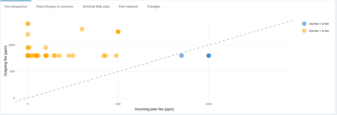
The dotted line is drawn across the diagonal where outbound fees equal the inbound fees, and colors are meant to give a quick visual of where the relationship sits. From the above graph, we can easily and quickly see that the node charges higher fees than its peers, and mostly at distinct rates, round number rates. Most of its peers charge less than 250ppm where it would charge roughly 2-3x that, in some cases the peer fee is less than 10ppm where the corresponding outbound fee is more than 1000ppm. This may be an indication the peer is a liquidity sink. In any case, it’s clear this node adopts an active rebalancing strategy based on its fees, which typically allows it to manage liquidity without generating much, or any, of a loss.
The peers-of-peers in common plot shows just that: the number of channel peers a node has in common with their other peers. Here’s an example:
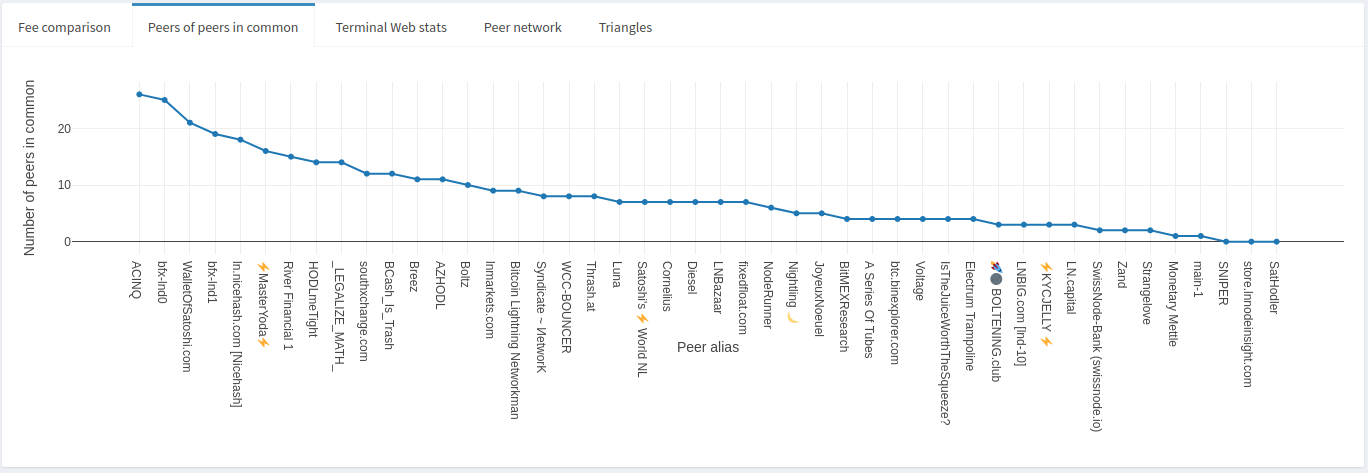
We can see from the plot that ACINQ has active channels with over 30 of this node’s peers, more than 60% of its peers! That’s not surprising given how big the ACINQ node is. This may be a good or a bad thing depending on a number of factors. From a routing node’s perspective it may not be ideal given how many potential paths lead through ACINQ that a channel to them would be redundant. On the other hand, it may be that many of ACINQ’s channels do not have liquidity where it is needed, thus maintaining a properly balanced channel to them would encourage forwards.
Lightning Terminal ranks of peers are also available for viewing. The most useful information that can quickly be identified is potentially problematic peers. Here are the Terminal ranks heuristics:
"maximum_disable_ratio": 0.25,
"minimum_active_channel_count": 10,
"minimum_stable_outbound_peers": 2,
"minimum_channel_age_blocks_count": 1000,
"minimum_median_capacity": 500000,
"minimum_routable_tokens": 500000,
"uptime_percentage": 0.995
From a routing node perspective, ideally you would want a peer who doesn’t suffer from too many disabled channels (preventing forwards), have at least a minimal amount of channels to increase potential for forwards, have somewhat large channels to handle liquidity demand, and maintain good uptime.
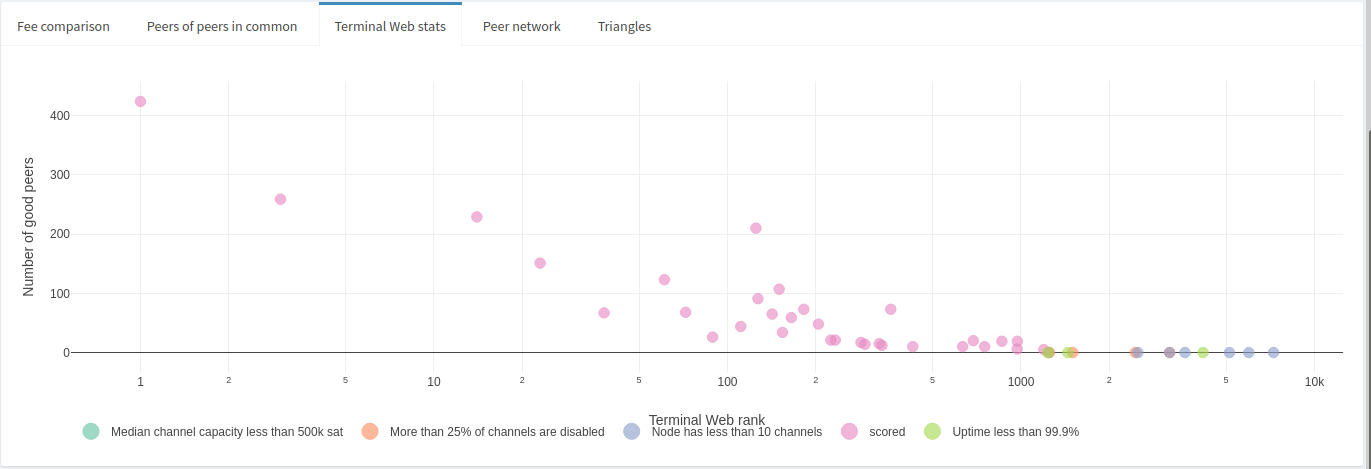
The node in this example appears to have peers that mostly meet the Lightning Terminal criteria. Only a handful are small nodes with fewer than 10 channels, and even fewer appear to be suffering some problem, like too many disabled channels or issues with uptime.
The Peer Network tab is a visual representation of the peers-of-peers-in-common tab. The node’s direct peers are displayed, as well as any channels that exist between those peers if hovering over any one of the peers. The line thickness is a rough indicator of channel size between peers.
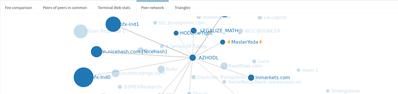
It can also be used to spot triangles between peers, which may be useful for visually identifying short rebalance routes that can initially be tried before reaching further out in the LN. The local graph also makes for a dope coffee mug design, made by sendnodes (disclaimer: this is an unpaid endorsement for a pleb making cool shit).
However, if you’re looking for a more systematic approach to identifying triangles, have a look at the Triangles tab which provides a searchable structured table.
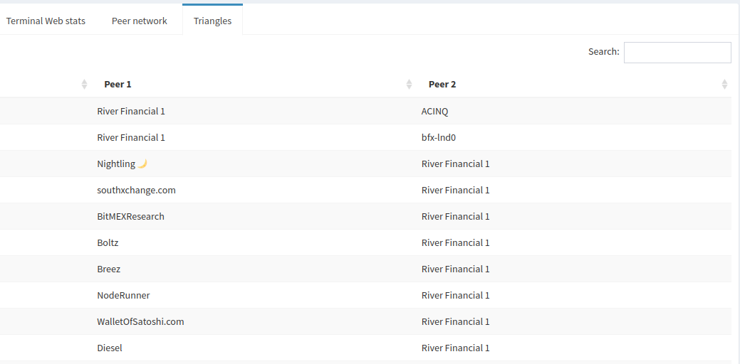
Coming back to how many peers ACINQ has in common with this node, that can be a good starting point to look for peers to make short routes for rebalancing if that’s your strategy.
That’s it for the Node Stats page. It’s a fairly dense page but a lot of information can be quickly gleaned from it.
2.3 Channel simulator
The channel simulator tool provides some insight into how a node’s position in the LN would change if a channel were to be opened or closed. The “impact” is measured in terms of centrality, more specifically betweenness, closeness and eigenvector centralities. There are a few dozen different algorithms that measure centrality from different perspectives, but the 3 mentioned here are the most basic and intuitive to make use of.
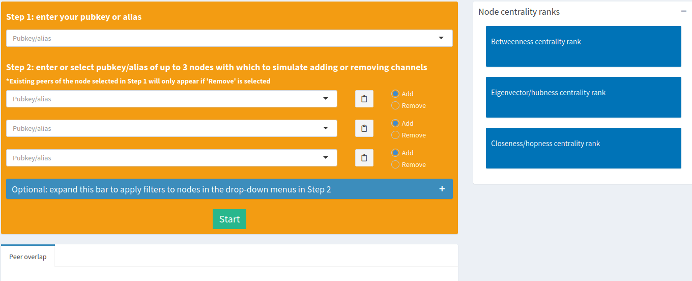
The tool can simulate opening, closing, or mixing opening and closing of channels for up to 3 nodes at the same time. You start by selecting your node of interest as the subject in the first step. Next, you’ll want to select up to 3 other nodes with which you want to simulate channel opens/closes. Upon selecting nodes, the tool will draw a Venn diagram for you indicating the number of peers each of the selected nodes have in common. This is a useful, quick visual to identify nodes that have a lot of overlap to possibly avoid, or keep for other purposes.
The drop-down menus to select target nodes contain a fairly comprehensive list of nodes (~8000) to select from, which can be overwhelming if you don’t already know which nodes you’re looking for. That’s why optional filters were included to help narrow down your searches if you were exploring.
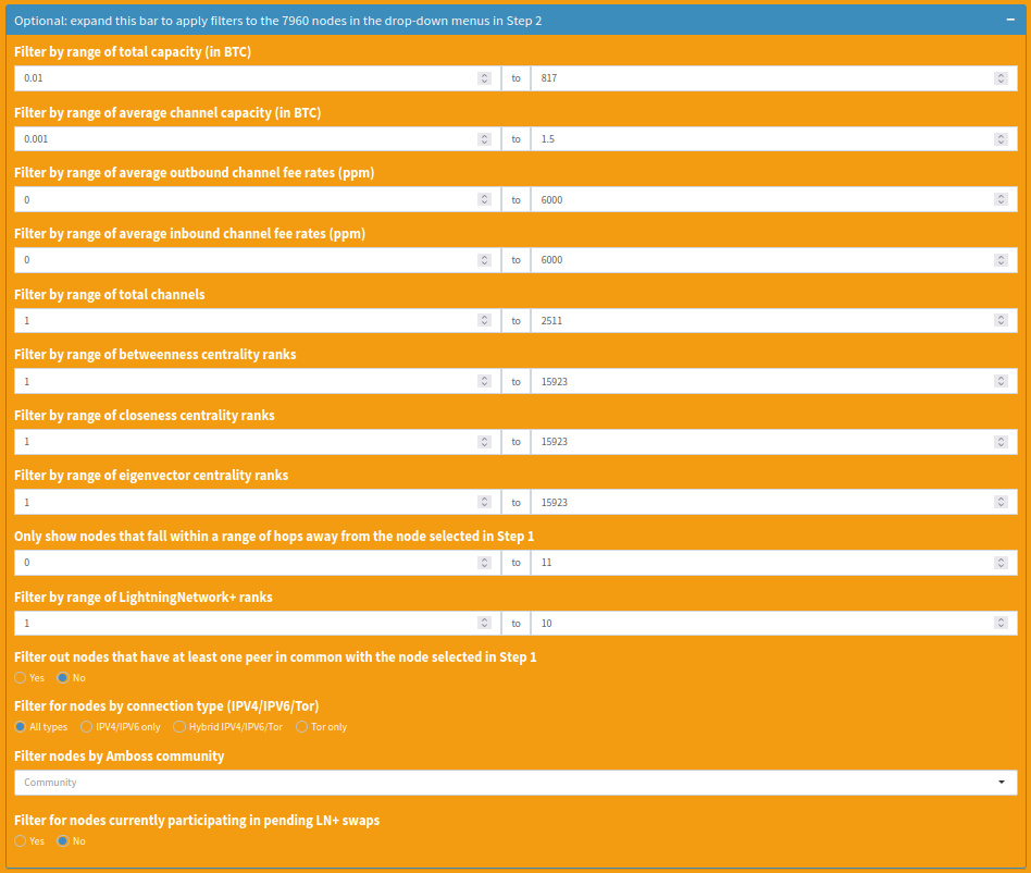
You have the option to filter by range of:
- total capacity
- average channel capacity
- average outbound fees
- average inbound fees
- number of channels
- betweenness rank
- closeness rank
- eigenvector rank
- number of hops away from the subject node
- LightningNetwork+ rank
- or filter out nodes that have at least one peer in common with the subject node
Additionally, there are more filters available after logging in to LNnodeInsight:
- network address type (IPV4/IPV6 only, hybrid Tor/IPV4/IPV6, Tor only)
- members of a specific Amboss community
- nodes participating in an active LightningNetwork+ swap
When filtering for nodes participating in an open LN+ swap, you’ll see a purple box indicating the channel size pop up underneath the ‘results’ box when you select a node from the target drop-down menus.
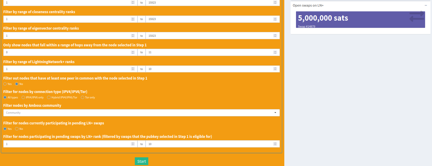
Clicking on that box will bring you directly to the swap page to quickly grab a spot!
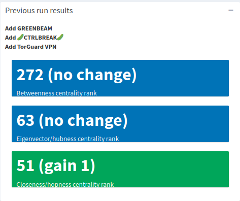
Once you’re ready to start a simulation, just hit the ‘Start’ button, wait a few moments, and you’ll see results like this:
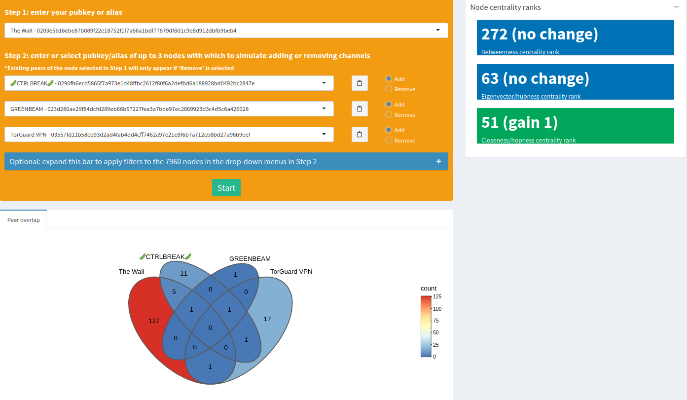
In thise case, the closeness centrality rank only improves by 1, so not the most ideal if you’re looking to optimize any one of those metrics. You could try another set of nodes, in which case you’ll see the results from the previous run pop up in a box just underneath the main results box as a reminder of what you ran.
2.4 Rebalance/payment simulator
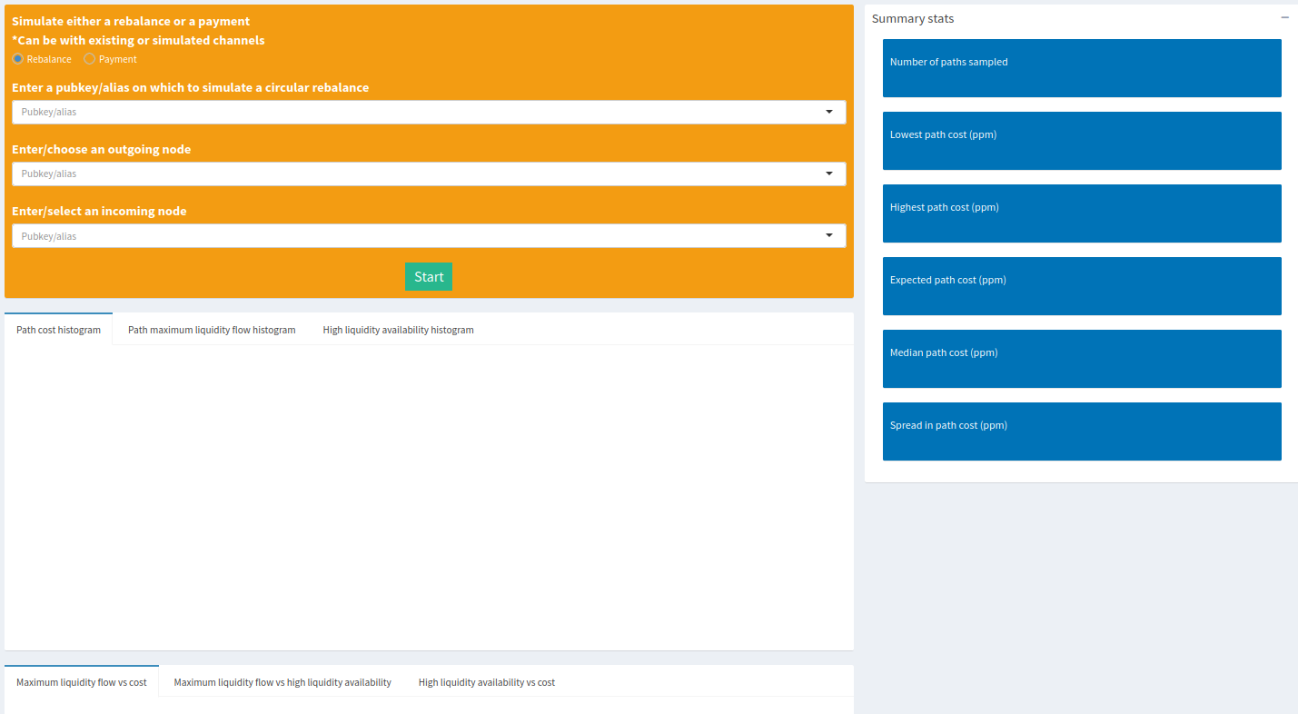
The rebalance (or payment) simulator is one of LNnodeInsight’s micropayment services (or unlimited use on subscription). It’s a quick way to get an idea of how much it might cost to rebalance (or pay) through a potential peer. Of course, it can be used for existing peers, but the real utility is in scanning rebalance or payment costs on candidate nodes before committing the sats to a channel. The only input required from you is to select the type of payment, either circular (rebalance) or one-way payment, your node pubkey (if rebalance), the “out” node and “in” node. Both outbound and inbound channels can be existing or potential. If a channel doesn’t exist between the starting node and the outbound or inbound node, then a channel will be simulated.
Once you’re satisfied with the input, hit the ‘Start’ button, then wait a minute or so for the results to come in. There’s a ton of information provided by this tool. Let’s start with the summary statistics pane. It provides a quick look at what came out of sampling paths between the outbound and inbound nodes.
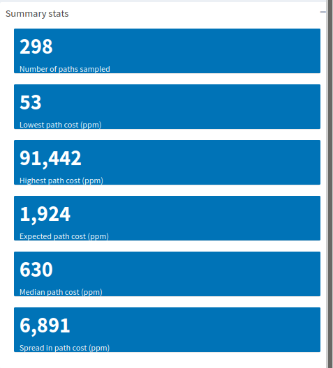
The default view includes summary stats about the path costs, but the statistics that get summarized change when you click on a different histogram tab. In any case, the summary includes:
- Number of paths sampled
- Minimum observed value
- Maximum observed value
- Mean value
- Median value
- Spread in the data
Typically the mean will be skewed higher than the median. We saw in the Build-Your-Own-Chart section that fees follow a sort of Pareto distribution, most nodes charge extremely little in fees whereas very few charge relatively high fees. What you can expect to pay in a rebalance is probably closer to the median value. Why so? The simplest assumption is that the cheapest paths will be exhausted of useful liquidity first, and the most expensive will be depleted last. Chances are that liquidity can be found on paths where the total cost falls in the mid ranges of the distribution. Pretty useful for just a few summary statistics, don’t you think? Let’s have a look at the path cost distribution itself:
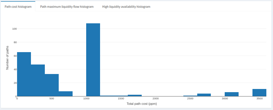
We can see the paths that cost more than 1600ppm are the ones skewing the average. There’s a big gap between those paths and the next cheapest group of paths, at around 1000ppm. That said, the effective paths are probably the ones around 1000ppm or less. Given the shape of those data, we’d hope for a 600ppm rebalance, but there’s also a good chance the next cheapest paths are closer to 1000ppm.
Since the tool samples fees along paths, we also get information about channel sizes along those paths. We can easily identify where bottlenecks can occur in terms of how large of a payment can flow. This concept is called maximum liquidity flow. It can also tell us where liquidity is most likely to be constrained as a function of fees. Click on the ‘Path maximum liquidity flow histogram’ tab and you’ll see the summary stats pane change as well. Here’s an example:
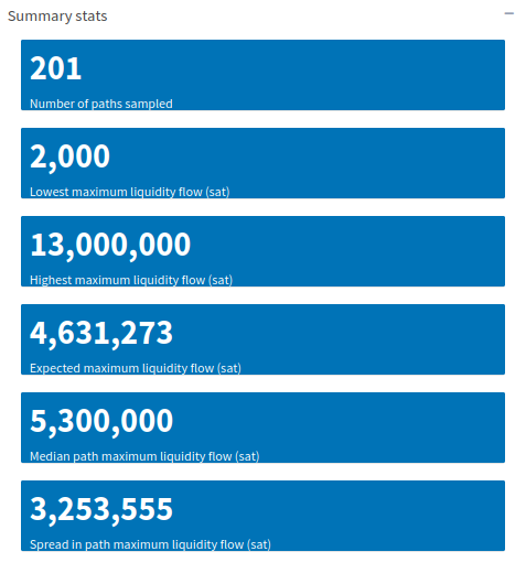
Here, the smallest channel size observed was 2000sats (extremely small, and not usable!), the highest was 13M sats (higher than normal). The median and mean channel sizes were fairly close to each other, around 5M sats. Here’s what the distribution looks like:
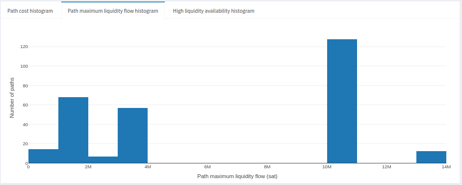
It looks like most channels in this sample were in the 10M sat range, and the remaining mostly in the 1M-4M sat range. What we can gather from this is that rebalances are most likely to test paths where the maximum liquidity flow is at least 1M sats. That’s a reasonable amount but we also assume that liquidity is where it needs to be. Channels at 1M or lower are the bottleneck here and it might be difficult to rebalance meaningful amounts at relatively cheap prices. Recall above that we might get lucky rebalancing at 600ppm, otherwise we’ll fall into the 1000ppm range. Depending on liquidity, it’s likely that we’ll be finding more expensive paths that have the liquidity we’re looking for. Speaking of liquidity availability, we also have a (limited) view on the liquidity availability. Let’s take a peek by clicking on the ‘High liquidity availability histogram’:
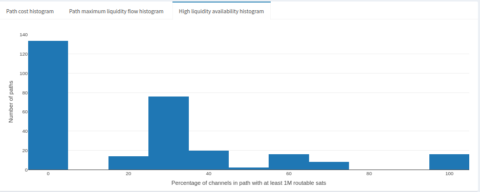
This plot shows us the proportion of channels in the sampled paths that most likely have good liquidity availability. It’s not perfect for the same reasons the node liquidity estimates are imperfect. In any case, we can still make reasonable guesses about liquidity distributions. We can tell that most paths either don’t have adequate liquidity or we don’t have information about them. Other paths fall in the 20-70% range, and very few have 100% known and adequate liquidity. Higher liquidity availability tends to be associated with higher channel fees. So the 20-70% range might also fall into the range of paths that cost 600-1000ppm.
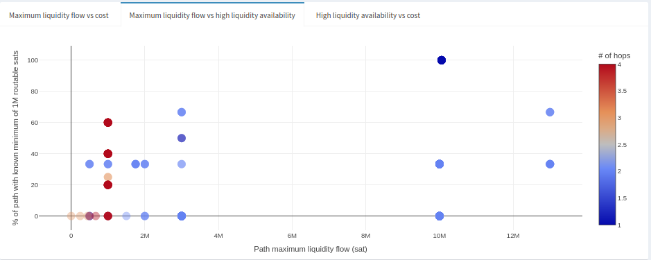
So far we’ve only looked at distributions of individual properties of the sampled paths. Now, we’d want to get an idea of the relationship between them. Let’s dive into the scatter plots, starting with the ‘Maximum liquidity flow vs cost’:
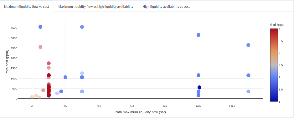
The first thing worth noting in this graph is the more hops we have to make in a path, the likelier it is we run into a small channel, and thus a liquidity bottleneck (that almost certainly doesn’t have the liquidity we want). However, we see that some paths have just 1 or 2 hops with relatively high maximum liquidity flow (>2M) at fees around 100-1000ppm range. Those look like promising candidates, but we would want to get an idea of liquidity availability first. They’re appealing paths so it’s likely the liquidity will have been bought up already.
This plot tells us that paths with maximum liquidity flow greater than 2M have known liquidity at least to some extent, few are known entirely, but some might not have liquidity at all. Let’s add a little more context to this result by looking at the cost of paths compared to high liquidity availability.
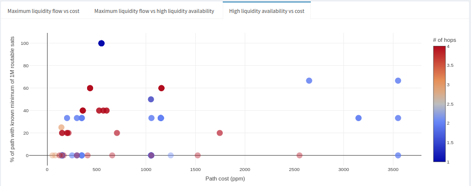
In this case, paths with more hops are also correlated with lower fees, but that also means that useful liquidity is most likely exhausted. Only a few paths with few hops at around 600ppm cost (consistent with what we saw in previous graphs) appear to have high liquidity availability. It’s impossible to tell if that will persist in time, but at least there are options. Otherwise, we start falling into the 1000ppm range, but liquidity is most likely more available in those cases given the cost.
That essentially covers all the information generated by this tool. To summarize this example: we would hope for a rebalance cost in the 600ppm range where we don’t see too many maximum liquidity flow constraints, and there’s evidence that liquidity is available at that cost range. Otherwise, we fall into the 1000ppm range. This might be an opportunity where maintaining a channel between these two nodes could potentially be profitable given the price gap between 600ppm and 1000ppm, provided liquidity can be maintained, your node is reasonably connected, and there’s liquidity demand between these two nodes.
2.5 Capacity-fee simulator
The capacity-fee simulator provides fee and channel capacity suggestions for a node. Two different fees are recommended, one for a passive fee strategy and one for an active fee strategy. These suggestions are meant to be either a starting point to set fees until enough time has gone by to better price liquidity, or as a fee valuation for an existing channel (see here for more details). Two different channel sizes are suggested depending on how much capital you’re looking to deploy in a channel. As a routing node, the minimally viable capacity is really the lower bound in order to make capital productive. It signifies the maximum liquidity flow determined along paths sampled in the simulator. Think of it as insurance against being a potential bottleneck in routes, but managing liquidity on such a small channel size can be difficult and this channel might even end up being a bottleneck anyway. Ideally, the minimum suggested capacity is the lowest you might want to go, more so for making liquidity management for tractable.
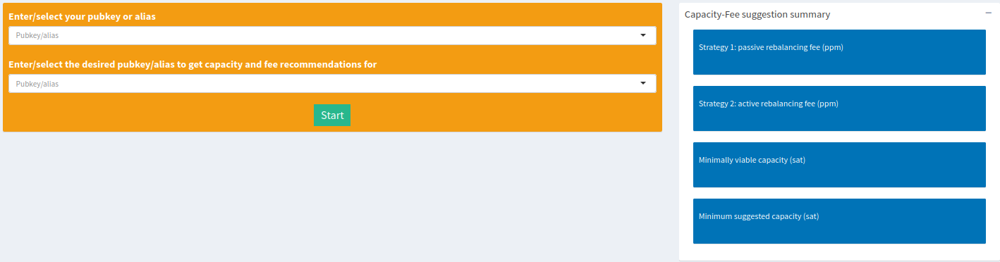
To start, enter your pubkey (or a pubkey of a different subject node where you’re considering opening a channel), and enter a target pubkey for which to get fee and capacity recommendations. The computation can take several minutes. You’ll end up with something like this:
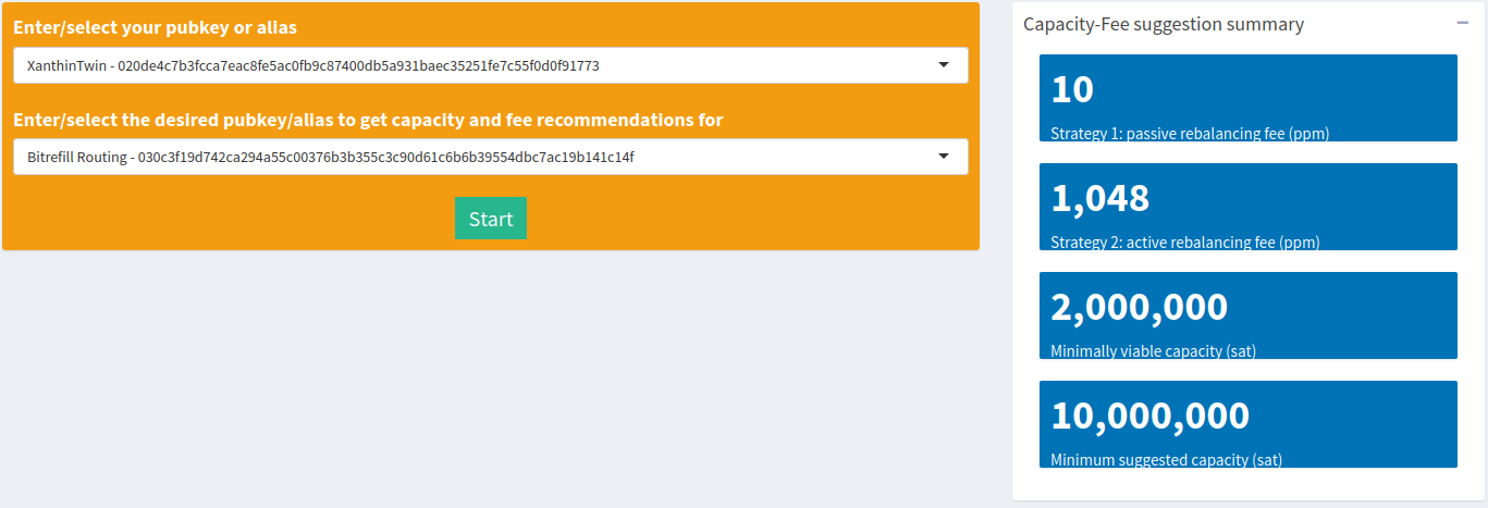
The passive suggested here is at a mere 10ppm. That’s basically saying that most nodes on paths to and from Bitrefill Routing charge almost nothing. On the other hand, the active fee is at 1048ppm. One interpretation we can draw from this result is that the gap between the two fee strategies implies that it can be fairly expensive to maintain liquidity, or barely profitable to let liquidity do its thing. Of course, if you have valuable inbound from somewhere that’s looking to use the Bitrefill Routing node then you’ll probably be able to charge more than the active fee, which would make it easier to maintain.
The node alias itself is telling you that its intended purpose was for routing. As such, it’s probably a better idea to go with the 10M minimum channel capacity, which is usually a good size for maintaining liquidity in sudden bursts. Recall that the typical maximum liquidity flow across any path in the LN is around 1M sats, the time it would take to drain in increments would provide enough buffer time to refill that liquidity. However, there’s also a market for large HTLCs, mostly between the extremely large nodes that are also exchanges. If you’re providing huge and valuable liquidity over a single hop between entities that typically need it then there’s a good chance a 10M channel would not be enough. Your routing data (successes & fails) will tell you that over time.
2.6 Automated reports
A lot of information is packed into the tools at LNnodeInsight, and it can be really informative to run them all by hand at least a few times. It can also get tedious, which is why we offer to automate a number of the tools under a paid subscription. Let’s dig into what the ‘Reports’ page looks like.
The first element is a table summary of automated channel simulation runs to identify the top 10 nodes that increase each of your centralities the most. For those top nodes, the capacity-fee simulator is also run to give you suggested starting fees and channel sizes.
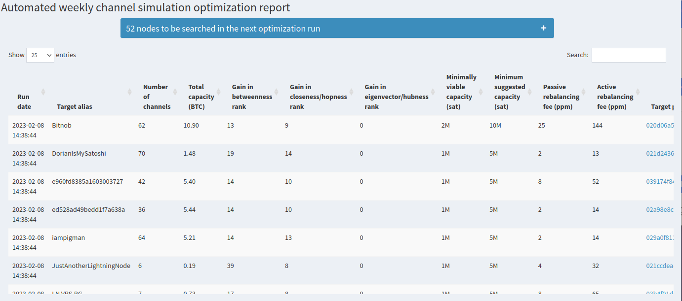
That table gets refreshed every 6 days around the time the subscription was activated. By default, we automatically look to optimize centralities in a list of around 3000 nodes. If you’re more interested in nodes that have specific properties, you can also apply filters to the automated runs just like the channel simulator. Each filter parameter you apply will show you how many nodes will be automatically searched.
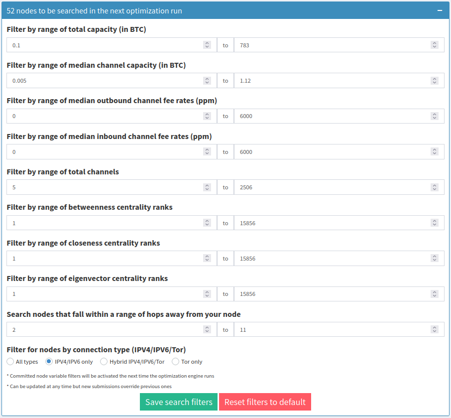
In this example, we filtered for nodes that are at least 2 hops away, is strictly on clearnet (IPV4/IPV6) and has a total capacity no greater than 783 BTC. That reduces the number of candidates drastically, down to 52. You’ll want to tune the filters to your liking. The filters will be applied to the next round of automated searches. Check back again around 6 days after the time listed in the ‘Run date’ column.
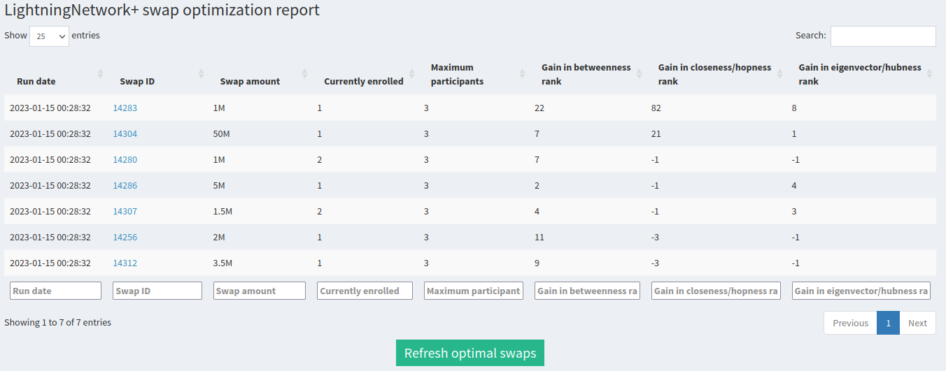
The next section contains a tool that, after hitting the ‘Start’ or ‘Refresh optimal swaps’ button, will automatically search all active swaps on LightningNetwork+ and propose optimal swaps that increase your centralities the most, just like the table above. It also includes some other useful information about the swaps, like the ID column which is a clickable link directly to the swap page, the swap amount, the number of currently enrolled participants and the total number of participants required for the swap. You can run this tool whenever you want, no need to wait!
The last section is the ‘Outbound liquidity value report’. It summarizes the results from automated runs of the capacity-fee simulator on all of your channels for both a passive fee and active fee strategy. Here’s what the passive fee histogram looks like:
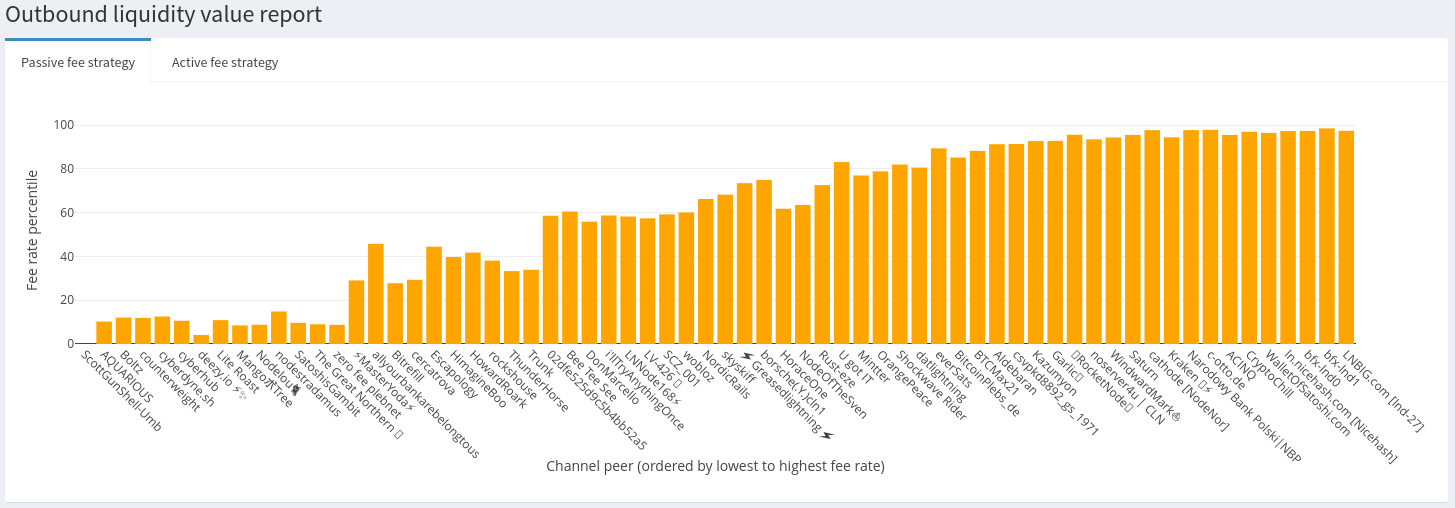
Each bar represents a node with which you have a publicly announced channel, ordered by outbound fees from lowest to highest. The height of the bar represents the percentile, from 0 to 100, on which it falls compared to other nodes in payment paths to and from the target. So, a channel fee of 1000ppm found to be in the 90th percentile implies that a fee of 1000ppm is more expensive than 90% of other nodes sampled in paths around the target. What does that mean? Well, if you’re seeing regular traffic at that fee rate then it is 90% more valuable (paired to the inbound channel) than others in a typical payment route. If you’re not seeing volume, then your outbound is overvalued.
From a passive strategy, about 1/3 of this node’s channels are deeply discounted compared to other channels in payment routes. Another 1/3 are much more expensive (>90th percentile for bfx-lnd0, bfx-lnd1, lnd-27, WalletOfSatoshi) than other channels in a payment route, assuming a passive strategy. What may be happening here is the higher priced channels are pulling all the liquidity, and the discounted channels are probably exhausted of useful liquidity.
Let’s look at the active fee histogram for contrast:
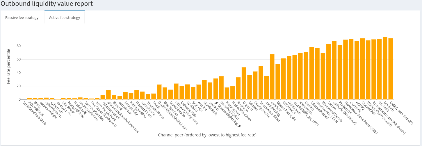
Just over 50% of this node’s channels are cheaper than at least 50% of other channels on payment routes. There’s no way this node could actively rebalance most of their channels without taking a heavy loss. The higher fees on nodes that tend to be liquidity sinks like the bfx nodes, WalletOfSatoshi and Kraken, are probably set to slow liquidity drain on the cheaper channels.
By comparing both the passive and active distributions We can tell that this node is trying to maintain two-way liquidity flow on their channels.
2.7 Sats4stats
Routing fees and selling channels are not the only sources of income possible for routing nodes. Information gathered by routing nodes is also valuable. LNnodeInsight is offering to buy routing node Mission Control data (currently limited to lnd nodes, other implementations in the future!). But why MC data? Liquidity tests are inherent to the LN right now. They’re needed to be able to maintain a routing node, which means liquidity tests are a form of work, and that Proof-of-Work has value.
The current market bid1 can be found on the front page of LNnodeInsight:
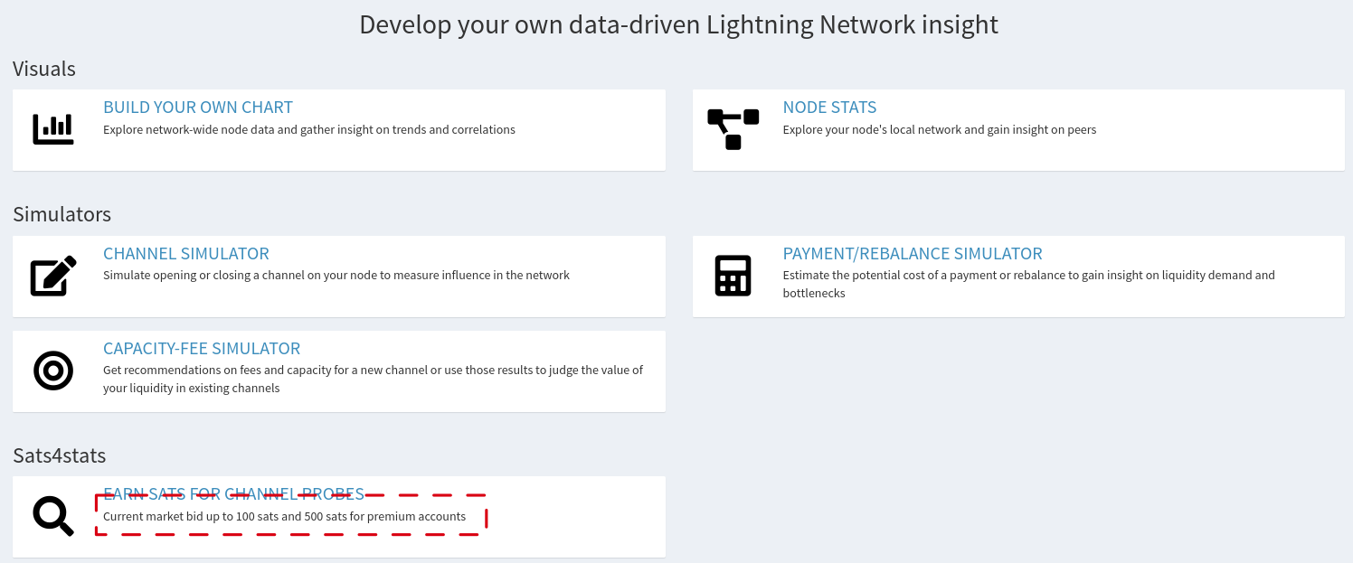
So how does it work? There are two ways to get sats4stats:
Either way, you’ll first need to login. If you’re using the API, you can generate a key on the ‘Account’ page. If you’re using a WebLN provider like Alby, head to the Sats4stats tab, and initiate the sale. Simple! Here’s a video demonstration:
Why give something away for free (or even throw it away!) when you can get paid for it?!
2.7.1 Which types of data can be sold?
We strive to be as transparent as possible with the type of data we are willing to buy, and what the implications are (privacy-wise and other), so that node operators can make well-informed decisions. Currently, we’re offering to buy Mission Control data, which is just a record of previous channel probes used to inform the pathfinding algorithm in making a payment. We encourage you to explore this data for yourself by running the querymc command with lncli (e.g., /path/to/lncli querymc). Here’s what a typical entry looks like:
{
    "node_from": "pubkeyA",
    "node_to": "pubkeyB",
    "history": {
        "fail_time": "0",
        "fail_amt_sat": "0",
        "fail_amt_msat": "0",
        "success_time": "0123456789",
        "success_amt_sat": "100",
        "success_amt_msat": "100000"
    }
}
This entry is telling us that we were able to successfully send 100 sats between pubkeyA and pubkeyB. Most importantly, we can see that:
- Probes does not reveal forwarding information
- Channel balances are not a feature of this data
- Payment outcome is not visible, in other words we don’t know if this probe is part of a payment that was successful or failed
- We don’t know if
pubkeyBis the destination or just a hop - Entries are disjointed from each other, therefore paths cannot be confidently reconstructed
Amounts subject to change↩